Factor theorem

lets say you substitute a value "a" into a polynomial P(x). well if that P(a) magicaly turns out to be equal to 0 that must mean that (x-a) will be a factor of that polynomial

imaginary numbers

Twil , a swimble, jucktillion, soomf , jiklet and quartizillion

The Gaussian integral

This is a wonderful integral that uses the gaussian function. It was first solved by Gauss, but the better and more clear solution was attributed to Poisson.

The Integral:

$$I = \int_{-\infty}^{\infty} e^{-x^2} \, dx$$

The first step is to square the integral. Weird I know, but just follow along. So we get:

$$I^2 = \int_{-\infty}^{\infty} e^{-x^2} \, dx \cdot \int_{-\infty}^{\infty} e^{-x^2} \, dx$$

Then, change the variable in the second integral:

$$I^2 = \int_{-\infty}^{\infty} e^{-x^2} \, dx \cdot \int_{-\infty}^{\infty} e^{-y^2} \, dy$$

Now, as they are two different variable, we can combine them to form one integral over the reals:

$$I^2 = \int_{-\infty}^{\infty} \int_{-\infty}^{\infty} e^{-x^2} \cdot e^{-y^2} \, dx \, dy$$

Since x and y are independent of one another, this combination won’t do anything to mess with each individual integral.

Next we can combine the exponents:

$$I^2 = \int_{-\infty}^{\infty} \int_{-\infty}^{\infty} e^{-(x^2+y^2)} \, dx \, dy$$

Now for the fun part!

We switch to polar coordinates. This means that x becomes:

$$x = r\cos(\theta)$$

And y becomes:

$$y = r\sin(\theta)$$

To visualise this, I have made this graph:

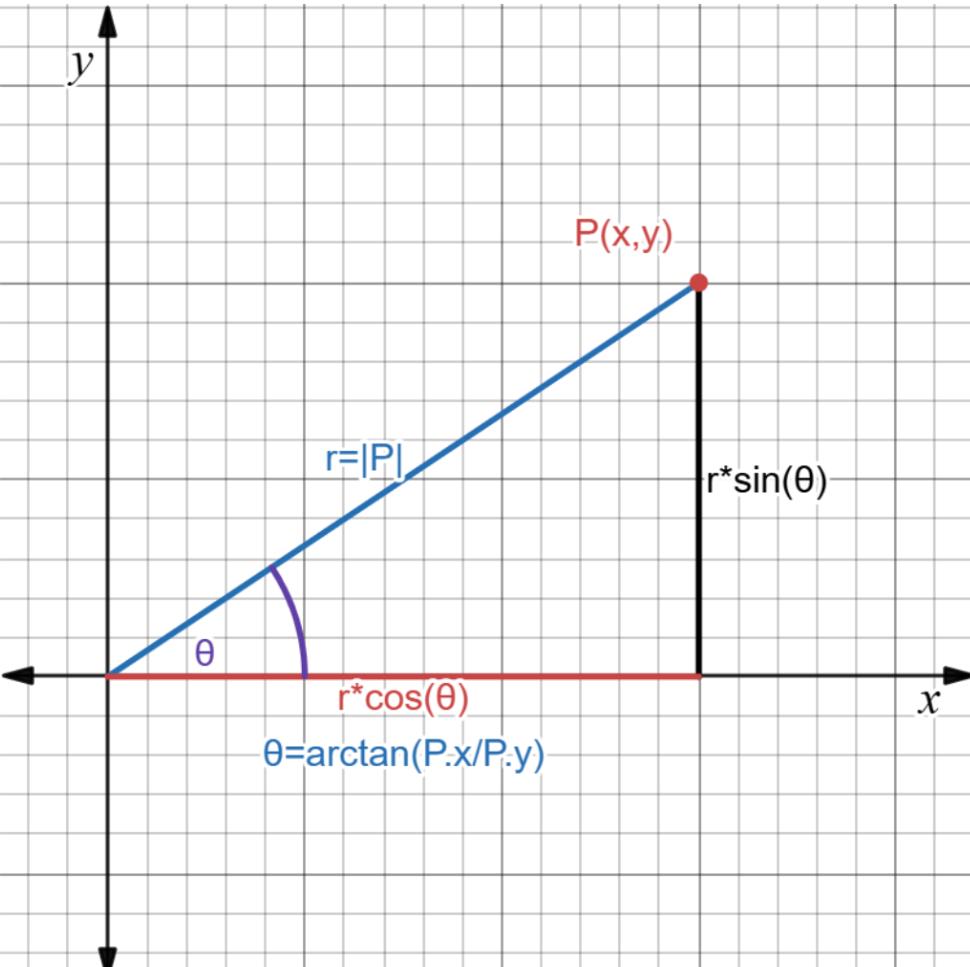
Now, the integral is still with respect to x and y. We must change this. It becomes:

$$dx\,dy = r\,dr\,d\theta$$

That extra r is known as the jacobian. I won’t get into it now.

We can now transform the integral into:

$$I^2 = \int_{0}^{2\pi} \int_{0}^{\infty} e^{-\left((r\cos(\theta))^2 + (r\sin(\theta))^2\right)} \cdot r\,dr\,d\theta$$

The bounds change for two reasons. 1. r can not be negative. It is strictly the magnitude of (x,y). 2.θ is only between 0 and 2π because it is the angles of a full circle in radians.

For the next step, we need to recall the identity:

$$\sin^2(\theta) + \cos^2(\theta) = 1$$

With some rearranging and cleaning, the integral becomes:

$$I^2 = \int_{0}^{2\pi} \int_{0}^{\infty} re^{-r^2} \, dr \, d\theta$$

Now, the inside integral is very easy to deal with because it is just the reverse chain rule.

$$\int_{0}^{\infty} re^{-r^2} \, dr = \frac{-e^{-r^2}}{2} \, \{0 \to \infty\}$$

Plugging in the values of the bounds we get:

$$\left(\frac{-e^{-\infty^2}}{2}\right) - \left(\frac{-e^{-0^2}}{2}\right)$$

I refuse to change the ∞ into a limit, I believe it should be treated as a number, but I digress.

The first exponent reduces to 0 as e raised to negative infinity is 0 (Once again I am ignoring limits). The second exponent becomes -1. This is then over the 2 so it becomes -1/2. But, the negative out front makes it positive.

The integral is now:

$$I^2 = \int_{0}^{2\pi} \frac{1}{2} \, d\theta$$

This is very simple and easy to deal with as its just the power rule:

$$\int_{0}^{2\pi} \frac{1}{2} \, d\theta = \frac{1}{2} \, \theta \, \{0 \to 2\pi\}$$

Plugging in the bounds, we get:

$$\left(\frac{1}{2} \cdot 2\pi\right) - \left(\frac{1}{2} \cdot 0\right)$$

This is just π on its own. I am not going to explain how to do basic arithmetic.

The integral is now:

$$I^2 = \pi$$

Now we square root both sides to get:

$$I = \sqrt{\pi}$$

We can ignore the negative value because we know that the gaussian integral is positive over the whole real line (exponents can’t be real for any real number)

We have now solved the gaussian and get this elegant integral solution:

$$\int_{-\infty}^{\infty} e^{-x^2} \, dx = \sqrt{\pi}$$

Wow! Isn’t that beautiful?

This integral has some very nice multivariable calculus parts. I think it’s pretty neat.

For an extra challenge, I recommend this integral:

$$\int_{-\infty}^{\infty} e^{-a \cdot x^2} \, dx$$

Where a is some constant greater than 0 (and real).

Jacobian Proof

In my proof of the Gaussian integral, I mentioned the jacobian when converting from cartesian to polar coordinates. I decided to skip over the details, so I will go through them now.

The Proof:

Let’s rewrite dxdy:

$$dx\,dy = dA$$

We call it dA because it’s an area.

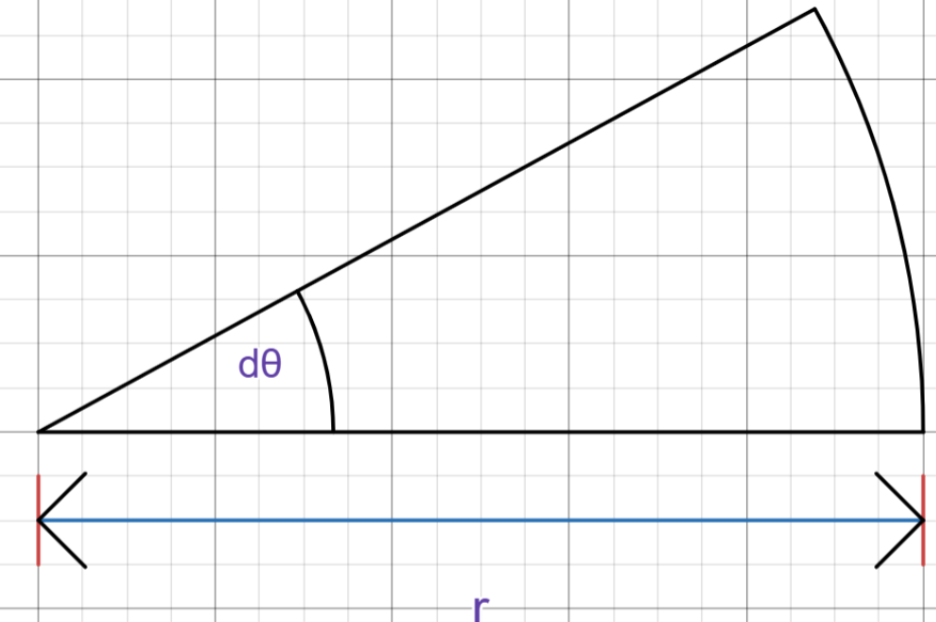
Now, picture a sector of a circle with radius r and angle dθ:

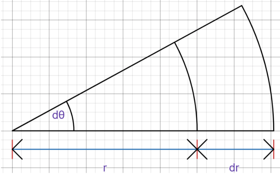
Next, picture a sector with a radius slightly bigger than this one, but with the same angle:

We’ll call that little area between the sectors dB:

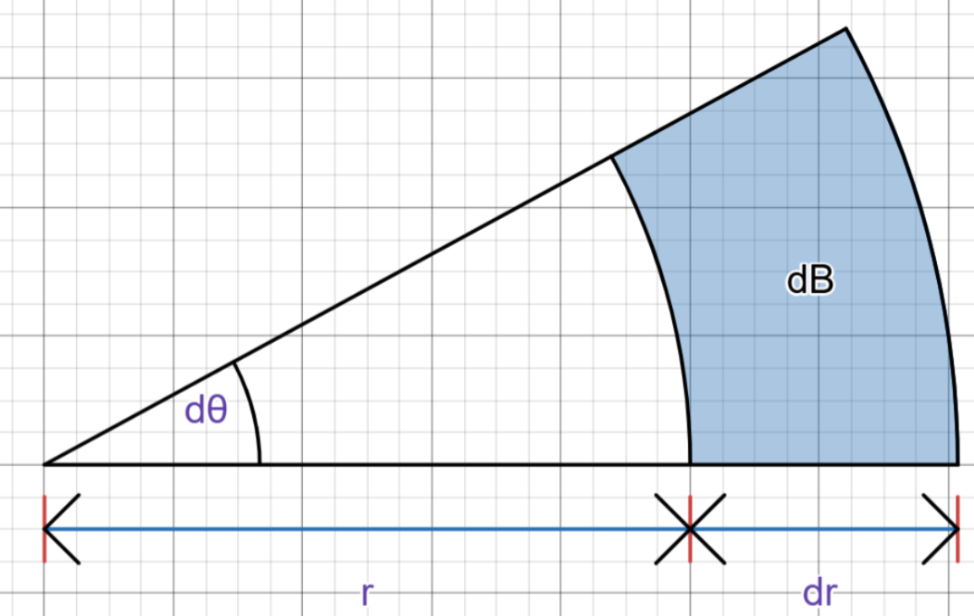
The area dB can be found by subtracting the area of the smaller sector from the larger sector:

$$dB = \frac{(r+dr)^2 d\theta}{2} - \frac{r^2 d\theta}{2}$$

Then through rearranging:

$$dB = \frac{d\theta}{2}\left((r+dr)^2 - r^2\right)$$ $$dB = \frac{d\theta}{2}\left(\left(r^2 + 2r\,dr + dr^2\right) - r^2\right)$$ $$dB = \frac{d\theta}{2}\left(2r\,dr + dr^2\right)$$ $$dB = r\,dr\,d\theta + \frac{dr^2\,d\theta}{2}$$

dr is already pretty small, so dr^2 is going to be VERY small. So small, in fact, we can just ignore it. This makes dB:

$$dB = r\,dr\,d\theta$$

Since dA and dB are incredibly small areas, we can say that they’re approximately equal to one another:

$$dA \approx dB$$

This now allows us to rewrite dxdy:

$$dx\,dy = r\,dr\,d\theta$$

Note: I replaced the “approximately equals” with an equals sign because at such a small scale they can just be written to be equal to one another.

Et voilà! That’s the proof. It’s not the most elegant. I had originally learnt it from a physicist friend of mine, so it's not trying to be rigorous. For the real proof there’s some matrix multiplication stuff that I don’t know all too well